Our Method

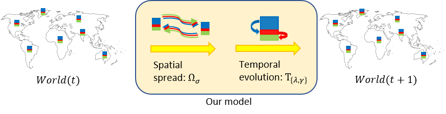
Effective modeling of epidemic spread requires modeling of: (a) the temporal evolution of a disease in a small population which mixes well, and (b) the spatial spread of the disease between large geographical areas (e.g. states and countries) across which the population only mixes by the virtue of explicit travel.

We propose a graph-based domain-knowledge informed model to capture disease transmission patterns from (potentially under-reported) heterogeneous spatiotemporal observations. Specifically, our approach combines: (a) a variant of the SIR compartment model to reflect the local temporal evolution of the epidemic, and (b) a diffusion operator characterizing the inter-state/country interactions to model the global spread of the epidemic. Our model parameters are learnt end-to-end from observed spatiotemporal data and provide interpretable visualizations of the spread dynamics.

Fig 1: Local population modeled by three compartments: Susceptible [S], Infected [I], Removed [R]

Fig 2: Model global population as a graph with nodes containing local populations in each of the three categories: [S, I, R]

Fig 3: Diffusion operator Ω_σ parametrized by σ models spatial spread between local populations at each time step.

Fig 4: Operator T_{λ,γ} parametrized by λ and γ models temporal evolution within a local population at each time step.

Fig 5: Our model combines spatial spread (global) and temporal evolution (local) operators to model the disease state in the world at each time step. Parameters (σ,λ,γ) are learnt end-to-end via gradient descent by minimizing prediction error for the total reported confirmed cases in all local populations at all time steps.

Modeling equations of our GraphSIR method

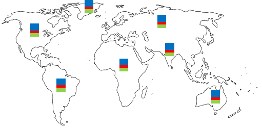
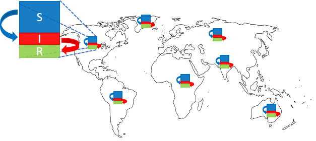
We denote the susceptible, infected and removed compartment populations on graph node $i$ at time $t$ as $S_i(t), I_i(t)$ and $R_i(t)$ respectively, s.t. $S_i(t) + I_i(t) + R_i(t) = N_i \forall t$, where $N_i$ is the total population at node $i$.

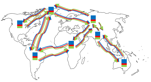
We define the population diffusion operator $\Omega$ on any compartment $A_i(t)$ ($A \in {S,I,R}$) to calculate how many people result on node $i$ due to spatial movements in a day:

$\Omega[A_i(t)] = A_i(t) + \sigma \sum_{j=1}^K \left( f_{ji} \frac{A_j(t)}{N_j} - f_{ij} \frac{A_i(t)}{N_i} \right),$

where $\sigma$ is a learnable transfer coefficient. Here $f_{ji} = f_{ij}$ is the average transport traffic between nodes $i$ and $j$. This can be estimated from data, e.g. flight or mobility data between nodes. Note that $\Omega$ preserves the density structure of the compartments and always sums them to $N_i$.

The temporal evolution is then defined by a standard SIR model:

$S_i(t+1) = \Omega[S_i(t)] - \lambda_i \frac{\Omega[S_i(t)]}{N_i} \Omega[I_i(t)]$ $I_i(t+1) = \Omega[I_i(t)] + \lambda_i \frac{\Omega[S_i(t)]}{N_i} \Omega[I_i(t)] - \gamma_i \Omega[I_i(t)]$ $R_i(t+1) = \Omega[R_i(t)] + \gamma_i \Omega[I_i(t)]$

Note that we use a separate spread rate and recovery rate $\lambda_i$ and $\gamma_i$ at each node since these can differ for instance in different countries or even amongst different states of the US.

We assume that we only observe an under-reported fraction of the total number of confirmed cases at each node over time, i.e. we observe $Z_i(t)$:

$Z_i(t) = \beta_i (I_i(t) + R_i(t)),$

where $\beta_i$ is the under-reporting fraction at node $i$.

We train our GraphSIR model end-to-end by minimizing the Mean Absolute Error Ratio (MAER) between our predicted values of daily confirmed cases ($Z_i(t)$) and the ground truth ($\hat{Z}_i(t)$):

$\min_{\{\lambda_i\}, \{\gamma_i\}, \{\beta_i\}, \sigma} \sum_{i=1}^K \sum_{t=1}^T \frac{| \hat{Z}_i(t) - Z_i(t) |}{\max(\hat{Z}_i(t), 1)},$

where the denominator serves to handle nodes with $0$ reported cases.

Modeling Influence of Intervention Policies

Since reliable intervention data is available for the US states, we additionally model the influence of intervention policies (e.g. stay at home) in our US spread prediction. Most intervention policies either impact the local spread of the disease at a node by reducing $\lambda$ or the global spread of the disease by reducing the travel coefficient $\sigma$. To model this reduction, we replace the $\lambda$ and $\sigma$ parameters with two learnable functions $\lambda(\cdot)$ and $\sigma(\cdot)$ of intervention. We respresent our policy on node $i$ at time $t$ with a binary variable $p_i(t)$ which is 0 when the policy had not been applied and turns to 1 when the policy is applied at the node. Since the effect of a policy is gradual, we use an exponential moving average of the policy denoted as $\hat{p}_i(t)$ as the to $\lambda(\cdot)$ and $\sigma(\cdot)$:

$\hat{p}_i(t) = \alpha \hat{p}_i(t-1) + (1-\alpha) p_i(t)$

This gives us $\lambda(\hat{p}_i(t))$ and $\sigma(\hat{p}_i(t))$ as:

$\lambda(\hat{p}_i(t)) = \lambda_{i,0} \exp{W_{\lambda} \hat{p}_i(t)}$ $\sigma(\hat{p}_i(t)) = \sigma_{i,0} \exp{W_{\sigma} \hat{p}_i(t)}$

where $W_{\lambda}$ and $W_{\sigma}$ are learnable parameters, while $\lambda_{i,0}$ and $\sigma_{i,0}$ are the base infection rate and transfer coefficient in the absence of intervention.